Liu C, Chen L C, Schroff F, et al. Auto-deeplab: Hierarchical neural architecture search for semantic image segmentation[C]//Proceedings of the IEEE Conference on Computer Vision and Pattern Recognition. 2019: 82-92.
1. Overview
1.1. Motivation
Existing methods focus on searching repeatable cell, while hand-designing the outer network strucuture which is not suitable for dense image prediction.
In this paper, it proposes Auto-DeepLab
1) Jointly search both inner cell level $\alpha$ and outer network level $beta$ based on gradient method (like darts)
2) Achieve same performance as DeepLabv3+ while 2.23 times faster.
3) 3 GPU days.
2. Methods

2.1. Cell Level Searching
1) $B$ blocks (two-branch strucuture) per cell.
2) The input set of $cell^l$ ($I^l$): {$H_l, H_{l-1}$}
3) The possible input set of $block_i$ in $cell^l$ ($I^l_i$): {$H_l, H_{l-1}, H^l_1, …, H^l_{i-1}$}, where $H^l_{i}$ is the output of $block_i$ in $cell^l$.
4) Each block contains $(I_1, I_2, O_1, O_2, C)$. Where $I_1, I_2 \in I^l_i$, $O_1, O_2 \in O$ means operators, $C \in \mathcal{C}$ means combination operator and simply use $\oplus$ in the paper.

2.1.1 Formulation
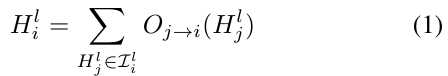
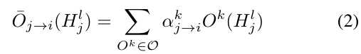

2.2. Network Level Searching
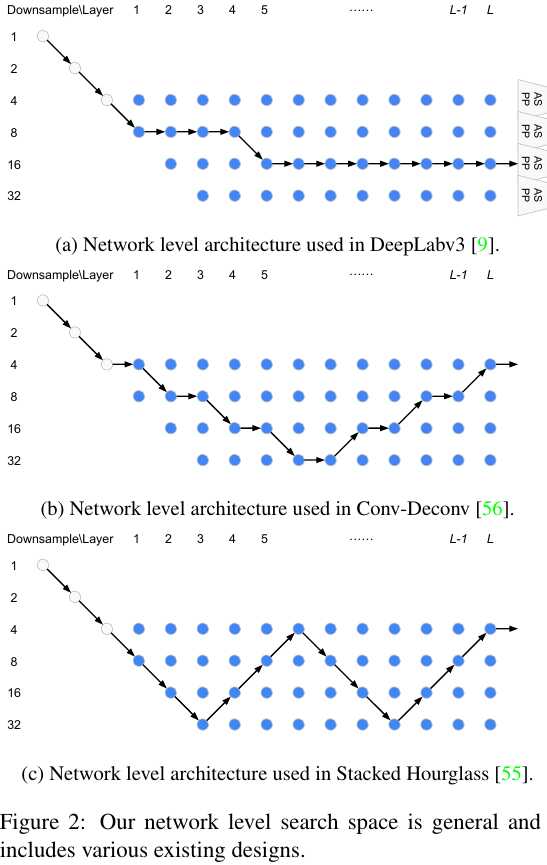
Two principles:
1) The spatial resolution of the next layer is either twice as large $\frac{s}{2} \to s$, or twice as small $2s \to s$, or remains the same $s \to s$.
2) The smallest spatial resolution is downsampled by 32.
1) Network begins with two-layer “stem”, each downsample by a factor of 2.
2) ASPP are attached to each spatial resolution at L-th layer. (simplify to 3-branch)
2.2.1. Formulation


1) Within a cell, all tensor are of the same spatial size.
2) Each layer $l$ will have at most 4 hidden states {$^4H^l, ^8H^l, ^16H^l, ^32H^l$}.
3) $\beta$ controls the outer network level.
4) Each $\beta$ governs an entire set of $\alpha$.
2.3. Optimization
Split the training data into $trainA$ and $TrainB$.
1) Update network weights $w$ by $\nabla_w L_{trainA}(w, \alpha, \beta)$.
2) Update architecture $\alpha, \beta$ by $\nabla_{\alpha, \beta} L_{trainB}(w, \alpha, \beta)$
2.4. Decoding
1) For cell level, retain 2 strongest predecessors for each block ($max_{k, O^k \ne_{zero}} \alpha^k_{j \to i}$). And “zero” means “no connection”.
2) For network level, choose the max $\beta$.

3. Experiments
3.1. Details
1)$L=12, B=5$.
2) $Filters=B \times F \times \frac{s}{4}$. $F=8$ is the filter multiplier.
3) Double the filter when half the resolution.
4) $\frac{s}{2} \to s$. stride 2 Conv of “double-half”.
5) $2s \to s$. Bilinear followed by $1 \times 1$ Conv.
6) 3-branch ASPP: only $3 \times 3$ Conv with atrous rate $\frac{96}{s}$. output filters of ASPP is still $B \times F \times \frac{s}{4}$.
7) Input image: random crop $321 \times 321$
8) $Batchsize=2, Epoch=40$.
9) SGD for $w$, Adam for $\alpha, \beta$
10) Find that if $\alpha, \beta$ are optimized from the beginning when $w$ are not well trained, the architecture tends to fall into bad local optima. So tart optimize $\alpha, \beta$ after 20 epochs.
3.2. Comparison


